Scaling Transformer Inference

Abstract

We’ve seen a major shift in the last few years: the release of ChatGPT largely settled the question of “Can we build large models?” Now, the focus has shifted to a far more practical (and often painful) question: “Can we run them efficiently?”

LLMs are good enough now. Research has matured over the last few years. Production systems are no longer prototypes; they’re high-traffic services answering millions of queries.

I’ve always been fascinated by how LLMs actually compute things. I knew the theory, the napkin math of the huge matrix multiplications, the insane amount of compute (theoretically) but I could never fully picture what was happening in practice. Imagine trillions of operations streaming through racks of accelerators, KV stores being looked up and updated, memory being paged in and out, and quantized tensors packing more compute into less silicon, all happening in the few hundred milliseconds between a user pressing Enter and the model answering. Makes me want to understand and answer the following question better.

How is inference THIS fast ?!?

So I went down the rabbit hole and documented what I learned, in the hope that it helps someone else avoid the same struggle.

In this post, I focus on the three bottlenecks that actually matter in production:

Throughput: The total number of tokens the system can generate per second across all users (critical for cost efficiency).
Latency: The time it takes to generate a single token for a specific user (critical for real-time chat).
Memory: How do we store and access huge context without collapsing the system.

We will walk through practical engineering patterns—KV caching and its tradeoffs, paged attention as a way to skirt the memory wall, and quantization techniques that squeeze models into affordable compute envelopes—and tie them back to real system design choices.

1. Introduction

As Moore’s Law suggests, gains in computational power have historically been exponential, but the parameter counts of modern models (spanning billions to trillions) have outpaced these hardware improvements.

Early advancements in Deep Learning primarily focused on training—struggling with the cost and time required to produce a model. Over the past few years, major research labs and industry leaders have developed techniques that make training large-scale models more manageable. As the training bottleneck eased, a new equilibrium pressure emerged: Inference.

But...What is inference?

For LLMs, inference involves:

Taking your input text (“prompt”)
Converting it into embeddings
Running it through all the model’s layers (lots of matrix multiplications + attention)
Producing the next token
Repeating this step-by-step until the final answer is complete

But...Why is it a challenge?

Lets discuss the background before we discuss why and how we solved this challenge.

2. Background: The Autoregressive Bottleneck

To understand the inference challenge, one must look at the underlying architecture of the Transformer (Vaswani et al., 2017). Unlike traditional neural networks that might process an entire input at once, LLMs are autoregressive. They generate text one token at a time.

To produce the 100th token, the model must essentially "re-read" or evaluate the context of all 99 previous tokens. If implemented naively, this leads to a quadratic computational cost O(n²) relative to the sequence length.

2.1 The "Naive" Inference Loop

To visualize why this is slow, consider this Python pseudocode representing the standard generation loop without optimization:

def generate_naive(prompt, max_tokens):
    tokens = tokenizer.encode(prompt)

    for _ in range(max_tokens):
        # Bottleneck: We re-process the ENTIRE sequence every time
        # even though we only care about the new token.
        # This function gets slower linearly as 'tokens' grows.
        q, k, v = compute_attention(tokens)

        next_token = sample(q, k, v)
        tokens.append(next_token)

    return tokenizer.decode(tokens)

In the code above, compute_attention(tokens) grows heavier with every step (as tokens increase). To reduce this redundant computation, the industry standard is a technique known as KV Caching.

2.2 The Two Phases of Inference: Prefill vs. Decode

Before diving into caching, it is vital to distinguish the two distinct phases of generation, as they stress hardware differently:

Prefill Phase (Compute-Bound): The model processes the user's input prompt (e.g., 500 words) all at once. This is a massive matrix multiplication operation that fully saturates the GPU's Compute Units (Tensor Cores). This determines the "Time to First Token" (TTFT).
Decode Phase (Memory-Bound): The model generates the response one token at a time. Here, the GPU is mostly idle, waiting for data to travel from memory to the chip. This determines the "Time Per Output Token" (TPOT).

Optimizations like KV Caching primarily target the Decode Phase.

2.3 The Mechanism of KV Caching

In the self-attention mechanism, the model computes three vectors for every token: a Query (Q), a Key (K), and a Value (V). The attention score is derived from the dot product of the Query with the Keys, which is then used to weight the Values.

\text{Attention}(Q, K, V) = \text{softmax}\left(\frac{QK^T}{\sqrt{d_k}}\right)V

When generating the next token, the Keys and Values for previous tokens do not change. Re-computing them is wasteful. Therefore, we cache these vectors in the GPU's High-Bandwidth Memory (VRAM).

Implementation View

Here is how the logic changes with a KV Cache. We only compute the query for the current token, and append the new keys/values to our growing cache.

class KVCache:
    def __init__(self):
        self.k_cache = [] # Stores keys for previous tokens
        self.v_cache = [] # Stores values for previous tokens

    def update(self, new_k, new_v):
        # We append only the new data, never re-computing old data
        self.k_cache.append(new_k)
        self.v_cache.append(new_v)
        return self.k_cache, self.v_cache

# The Optimized Loop
cache = KVCache()
for _ in range(max_tokens):
    # Only compute Q, K, V for the ONE new token
    q_new, k_new, v_new = compute_single_token(current_token)

    # Retrieve history from memory, not compute
    k_past, v_past = cache.update(k_new, v_new)

    # Attention now only looks at the cached list + new token
    next_token = attention(q_new, k_past, v_past)

While this reduces computational complexity, it moves the bottleneck to Memory Capacity. The self.k_cache list grows linearly. For long-context models (e.g., processing a 100-page document), this list becomes massive. For a 70B model with a 4096 token context, the KV cache alone can consume gigabytes of VRAM per user, causing the GPU to run out of memory (OOM).

3. Technical Discussion: Findings on Memory Management

3.1 The Problem of Contiguous Memory

My research into the state-of-the-art prior to 2023 highlights a significant inefficiency in how Deep Learning frameworks (like PyTorch) handled memory. Systems like NVIDIA’s FasterTransformer or the original Orca paper (Yu et al., 2022) relied on contiguous memory allocation.

Most tensor operations expect data to lie next to each other in physical memory to allow for fast vectorization. Because the length of an output response is unknown (a user might answer "Yes" or write a 2,000-word essay), these systems had to "reserve" a contiguous block of VRAM based on the maximum possible sequence length.

This leads to fragmentation, similar to hard drive fragmentation in the 90s:

Internal Fragmentation: If a slot is reserved for 2048 tokens but the user only generates 50, the remaining space is wasted.
External Fragmentation: As requests of different sizes finish and release memory, the VRAM becomes a "checkerboard" of free and used space. A new large request might be rejected even if total free space is sufficient, simply because there is no single continuous gap large enough.

Findings indicate that in these legacy systems, 20% to 80% of GPU memory was wasted due to fragmentation.

3.2 The Solution: PagedAttention (vLLM)

The most novel idea introduced in recent literature is PagedAttention, popularized by the vLLM library developed by researchers at UC Berkeley (Kwon et al., 2023).

Conceptualizing PagedAttention

Kwon et al. recognized that this was exactly the same problem Operating Systems faced in the 1960s regarding RAM usage. The solution then was Virtual Memory Paging. PagedAttention applies this to LLMs. Instead of demanding a contiguous block of physical memory, it divides the KV cache into fixed-size "blocks" (e.g., 16 tokens).

We can visualize PagedAttention not as a contiguous array, but as a Hash Map (or Block Table) that maps a logical sequence to scattered physical locations. The Attention kernel is rewritten to "walk" this table, fetching blocks from wherever they exist in memory.

# Traditional Attention (Contiguous)
# memory = [Tok1, Tok2, Tok3, Tok4, ..., Empty, Empty] (Must be one block)

# PagedAttention (Non-Contiguous)
# We can store chunks anywhere they fit, just like saving a file to a fragmented hard drive.
physical_memory = {
    "Block_A": [Tok1, Tok2],    # Stored at address 0x100
    "Block_B": [Tok3, Tok4],    # Stored at address 0x900
    "Block_C": [Tok5, ... ]     # Stored at address 0x200
}

# The Block Table acts as the "Translation Layer"
block_table = {
    "User_Request_1": ["Block_A", "Block_B", "Block_C"]
}

Key Advantages:

Zero Internal Fragmentation: Memory is allocated on-demand, block by block. The only waste is the unused space in the very last partially-filled block.
Memory Sharing (Copy-on-Write): This is crucial for advanced decoding like Beam Search or Parallel Sampling. If a user asks a chatbot to "Generate three different emails," the system does not copy the prompt three times. All three requests point to "Block_A" and "Block_B" in the block table, only allocating new unique blocks when their generated outputs diverge.

3.3 Quantization: Solving the Memory Wall

Parallel to better memory management is the compression of the data itself. Solving fragmentation is only half the battle; the other half is reducing the sheer volume of data we need to move. This necessity has driven a rapid migration from traditional FP16 (16-bit floating point) weights to highly compressed INT8 and INT4 (4-bit integer) formats.

To learn more - Quantizing LLMs - How & Why (8-Bit, 4-Bit, GGUF & More)

3.3.1 The "Memory Wall" Bottleneck: Arithmetic Intensity

Why does file size matter for speed? It comes down to Arithmetic Intensity—the ratio of calculations (FLOPS) to memory traffic (Bytes).

Training has high arithmetic intensity (lots of math per byte loaded).
Inference (Decode) has low arithmetic intensity. We load a huge weight matrix just to multiply it by a tiny vector (the single new token).

In modern GPUs (like the NVIDIA H100), compute power has increased vastly faster than memory bandwidth. The GPU spends most of its time waiting for data to arrive. Quantization attacks this directly. By reducing the weight size, we effectively increase the bandwidth.

To illustrate the scale of savings, consider this back-of-the-envelope calculation for a 70 Billion Parameter Model:

def calculate_vram(params_billions, precision_bits):
    bytes_per_param = precision_bits / 8
    total_gb = (params_billions * 1e9 * bytes_per_param) / 1e9
    return total_gb

# Standard FP16 (16-bit)
vram_fp16 = calculate_vram(70, 16) # ~140 GB
# (Requires expensive server-grade A100/H100 clusters)

# Modern INT4 (4-bit)
vram_int4 = calculate_vram(70, 4)  # ~35 GB
# (Fits on a single high-end workstation card)

3.3.2 Visualizing Quantization Code

To understand what is actually happening to the numbers, consider this simulation of Absmax Quantization. We scale the weights into the range of -127 to +127 (INT8) to save space, then "de-quantize" them on the fly when we need to do the math.

import numpy as np

def simulate_quantization(weights_fp16):
    """
    Simulates compressing weights from 16-bit float to 8-bit integer.
    """
    # 1. Find the maximum absolute value in the tensor
    max_val = np.max(np.abs(weights_fp16))

    # 2. Calculate the scale factor
    # (We map the max_val to 127, the max value of an 8-bit integer)
    scale = 127 / max_val

    # 3. Quantize: Scale and round to nearest integer
    weights_int8 = np.round(weights_fp16 * scale).astype(np.int8)

    # This 'weights_int8' is what we store in VRAM (4x smaller!)
    return weights_int8, scale

def dequantize(weights_int8, scale):
    # 4. De-quantize: Convert back to float for calculation
    return weights_int8 / scale

Conceptualizing Accuracy Preservation (AWQ)

A common concern is that "rounding down" numbers will make the model "dumber." Naive quantization (simply rounding every number) does indeed hurt performance. However, newer methods like Activation-Aware Weight Quantization (AWQ) use a smarter approach.

Imagine a sentence where specific keywords carry 90% of the meaning, while articles like "the" or "a" carry very little. If you blur the articles, the sentence is still readable. If you blur the keywords, it becomes gibberish.

AWQ identifies that in a neural network, not all weights are equal. Approximately 1% of the weights are "salient" (crucial) because they interact with large activation values. AWQ protects this 1% by keeping them in higher precision or scaling them specifically to preserve their information, while aggressively compressing the other 99%. This allows for massive speedups and memory savings with negligible loss in the model's intelligence.

4. System Design: Anatomy of an Inference Request

To truly understand how these optimizations function all together - in harmony, let us construct a mental image of how does a single request travel through a modern inference server. Imagine we are running a 70B Parameter Model (quantized to INT4) and a user sends a prompt.

Here is the lifecycle of that request:

Step 1: Arrival & Prefill (The Compute Spike)

The user sends a 500-token prompt. The system enters the Prefill Phase.

The Action: The GPU wakes up and processes all 500 tokens in parallel. This is a massive matrix multiplication event.
System State: The Tensor Cores are at 100% utilization. We are Compute-Bound.
Memory Role: The system calculates the Key and Value vectors for these 500 tokens.

Step 2: Allocation (The Operating System Layer)

Instead of reserving a massive, contiguous chunk of VRAM for the answer (which we don't know the length of yet), PagedAttention intervenes.

The Action: The system allocates small, non-contiguous "pages" (blocks) of memory scattered across the VRAM to store the KV cache for the prompt.
The Result: No memory is wasted on empty space. The "Block Table" records where these scattered pieces live, ready for retrieval.

Step 3: The Decode Loop (The Memory Grind)

The model begins generating the answer, token by token. We are now in the Decode Phase.

The Bottleneck Shift: The Tensor Cores are now mostly idle. The speed limit is no longer math; it is how fast we can move data.
The Fetch: To generate Token #501, the GPU requests the KV data for the previous 500 tokens. It uses the Block Table to hunt down the pages scattered in VRAM.
The Compression Win: Simultaneously, the model weights must be loaded. Because we used INT4 Quantization, the weights traveling from VRAM to the chip are 4x smaller than the full 16-bit precision weights. They arrive 4x faster, effectively quadrupling our bandwidth.

Step 4: Compute & Update

De-quantization: As the compressed weights hit the chip's registers, they are instantly converted back to high-precision (FP16) for the actual calculation.
Finalization: The math completes, the next token is chosen, and its specific KV data is written to a new page in memory.

This cycle repeats itself Fetch -> De-quantize -> Compute -> Store until the response is complete. To better understand this, let’s use the latest Gemini 3 Pro Nano Banana to create a visual representation of the inference lifecycle.

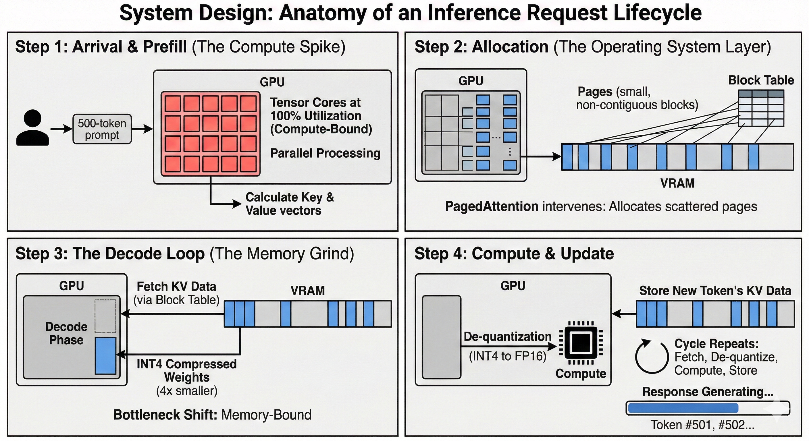
Diagram showing the lifecycle of an LLM inference request. — Figure 1: The journey of a single inference request.

5. Few Interesting Reads

Based on this review, the path forward for Transformer inference involves few key areas of research and application:

Speculative Decoding:
- Concept: In many sentences, the next word is obvious (e.g., "New York [City]"). Using a massive 70B model to predict "City" is a waste. Speculative Decoding uses a tiny, fast "Draft Model" to generate 5-10 tokens cheaply, and then the large "Target Model" verifies them all in a single parallel step.
- To learn more - Faster LLMs: Accelerate Inference with Speculative Decoding
Long-Context Optimization (Ring Attention):
- Concept: As context windows grow to 1M+ tokens (e.g., Gemini 1.5), even PagedAttention struggles with the sheer volume of KV cache. Ring Attention distributes the KV cache across multiple GPUs in a ring topology, allowing the context to be larger than the memory of any single card.
- To learn more - Ring Attention with Blockwise Transformers for Near-Infinite Context

6. Conclusion

We started this exploration asking "Can we run it efficiently?", but the answer revealed a deeper truth about the state of AI. The era of purely algorithmic wins—where a better model architecture solves everything—is pausing. We are re-entering an era of systems optimization, reminiscent of the early days of computing where every byte and cycle mattered.

If there’s one message to leave with, it’s this: Stop treating the GPU as an abstraction.

Today, the most impactful progress happens at the intersection of logic (the model) and physics (the memory bandwidth). We’ve learned that “intelligence” isn’t limited by how many parameters we can fit into a model—it’s limited by how fast we can move those parameters from memory to the compute units.

Thinking in systems terms changes everything. When a model feels slow, the right question isn’t “Why is it bad?” but “Is it compute-bound (prefill) or memory-bound (decode)?”

Efficiency is what turns a supercomputer demo into a feature on your phone. As we push toward multi-modal models and AI Agents, the "software" of memory management will become the defining constraint of the "hardware" of intelligence.